
If you’re looking for additional Excel pointers, we’ve put together guides on how to password protect an Excel document and how to make a graph in Excel.
Select All
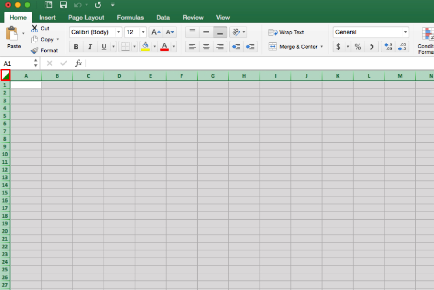
If you want to highlight a specific grid of cells, you can simply click and drag, but what if you want to select all of them? There are two ways. You can use the keyboard shortcut — Ctrl + “A” in Windows 10, Command + “A” in MacOS High Sierra and earlier iteration of MacOS — or go to the smaller cell in the upper-left corner (marked by a white arrow) and click it.
How to shade every other row
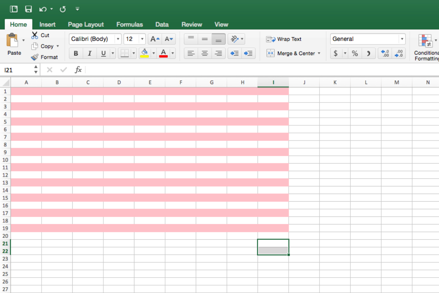
Spreadsheets can be awfully drab, and if you’ve got a lot of data to look at, the reader’s eyes might start to drift aimlessly over the page. Adding a splash of color, however, can make a spreadsheet more interesting and easier to read, so try shading every other row.
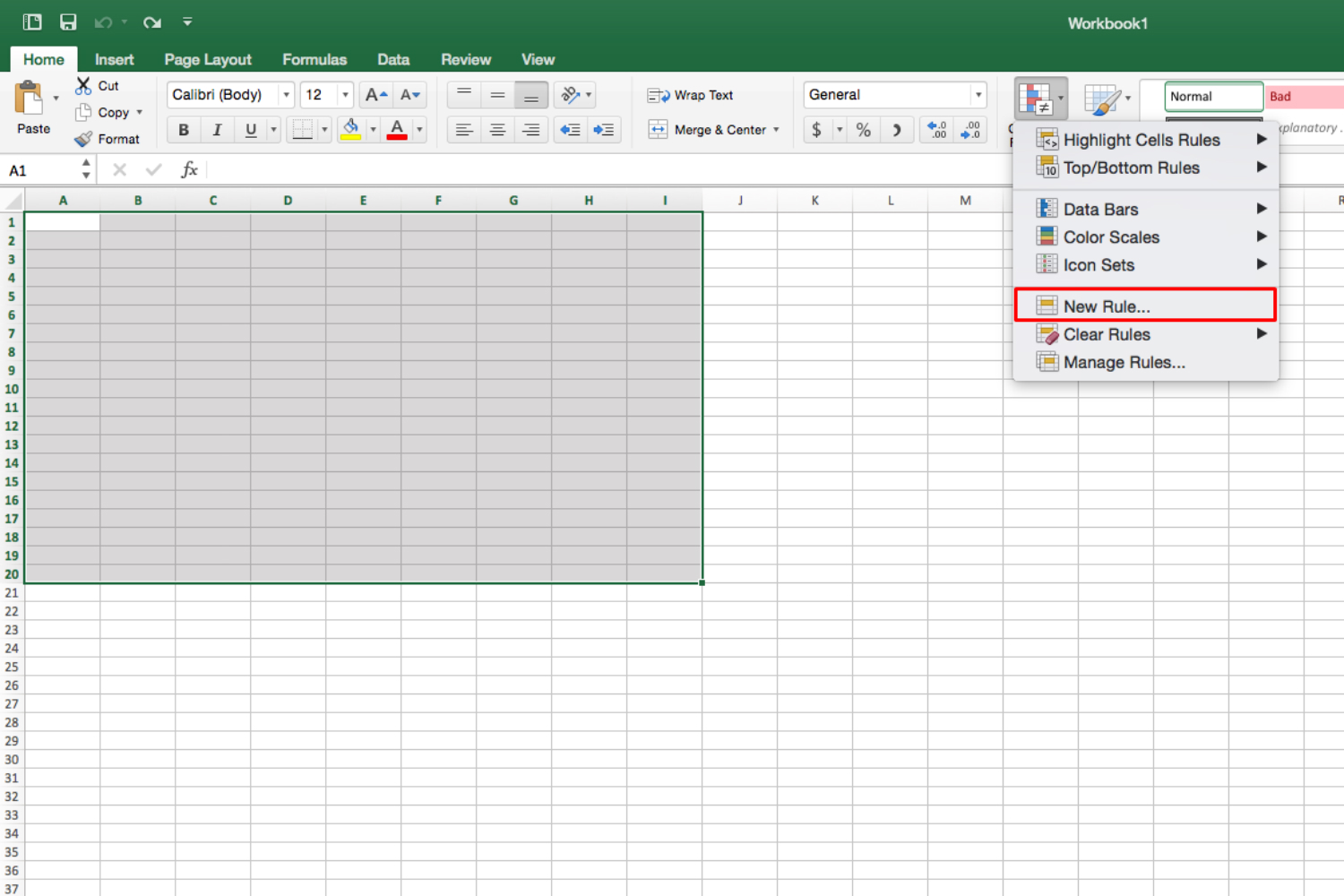
To start, highlight the area you want to apply the effect to. If you want to add color to the entire spreadsheet, just select all. While viewing the Home tab, click the Conditional Formatting button. Then, select New Rule from the resulting drop-down menu.
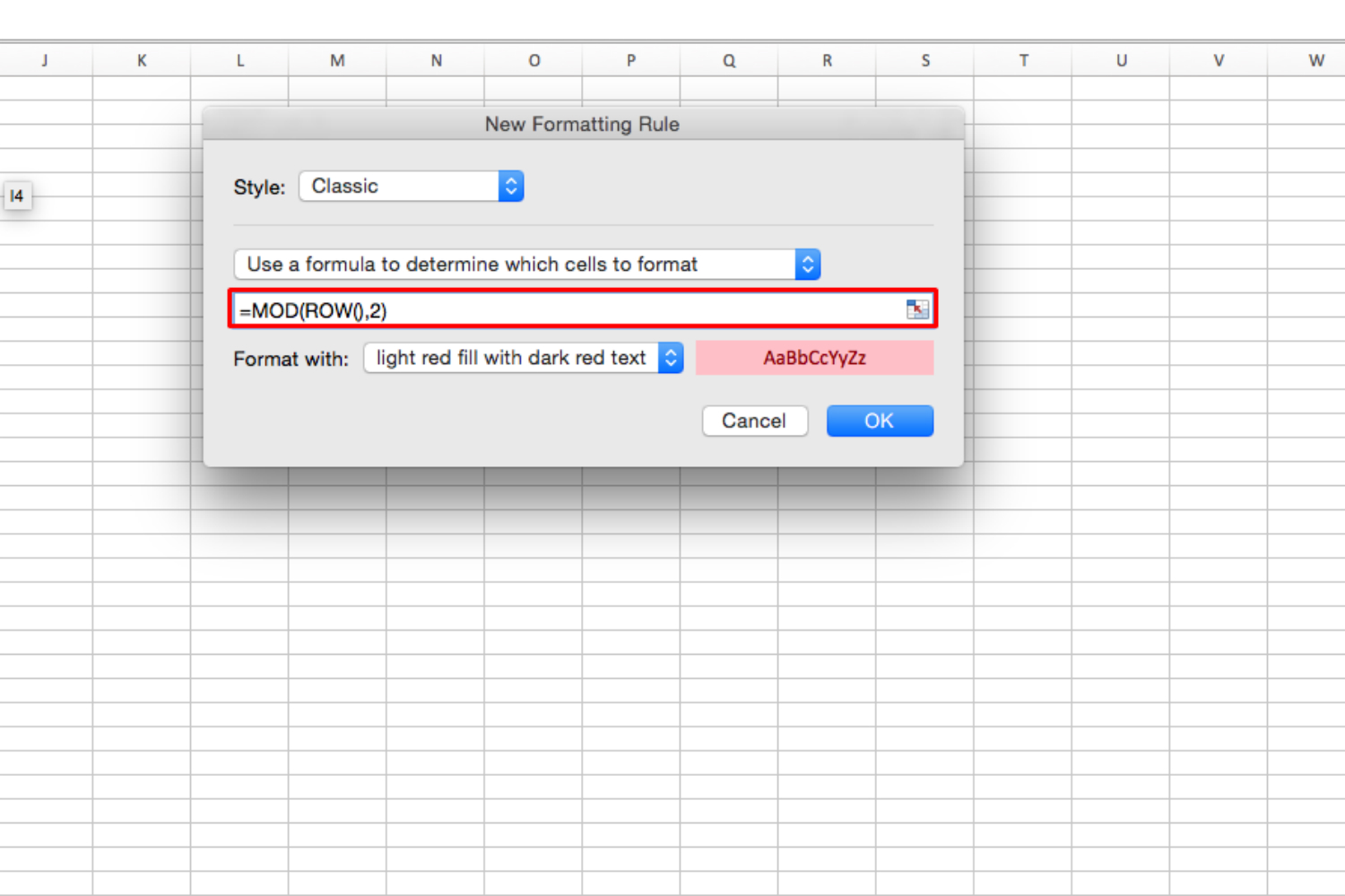
In the Style drop-down menu, choose Classic.
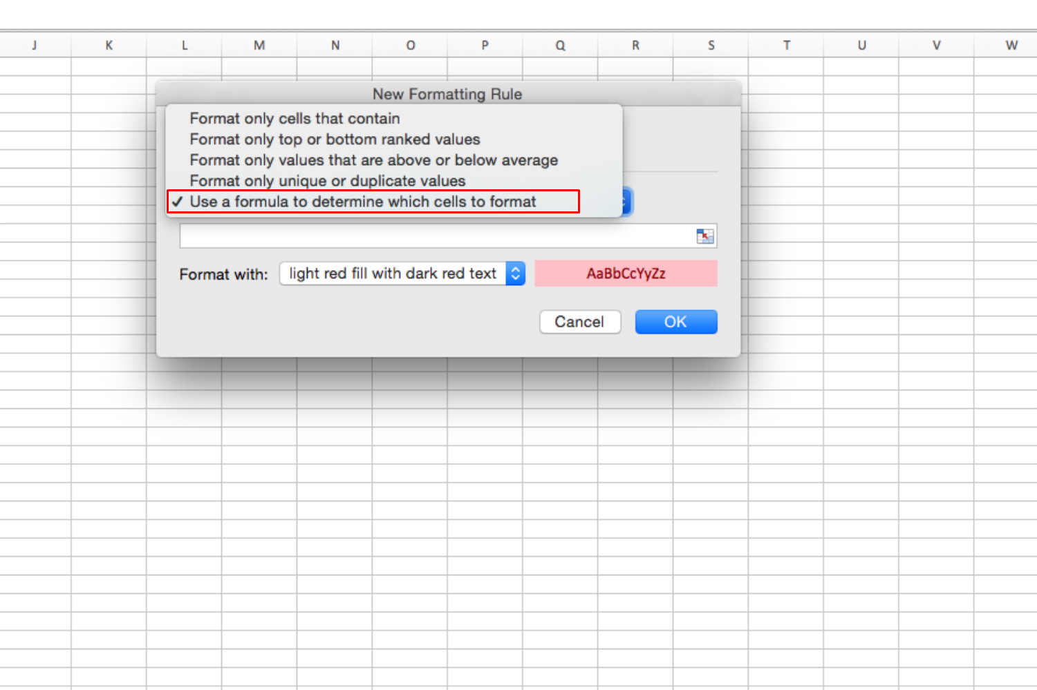
Afterward, select Use a formula to determine which cells to format.
The formula to enter is “=MOD(ROW(),2).”
Choose which fill color you want, then click OK. Now the rows should be shaded in alternating color.
Hide/unhide rows
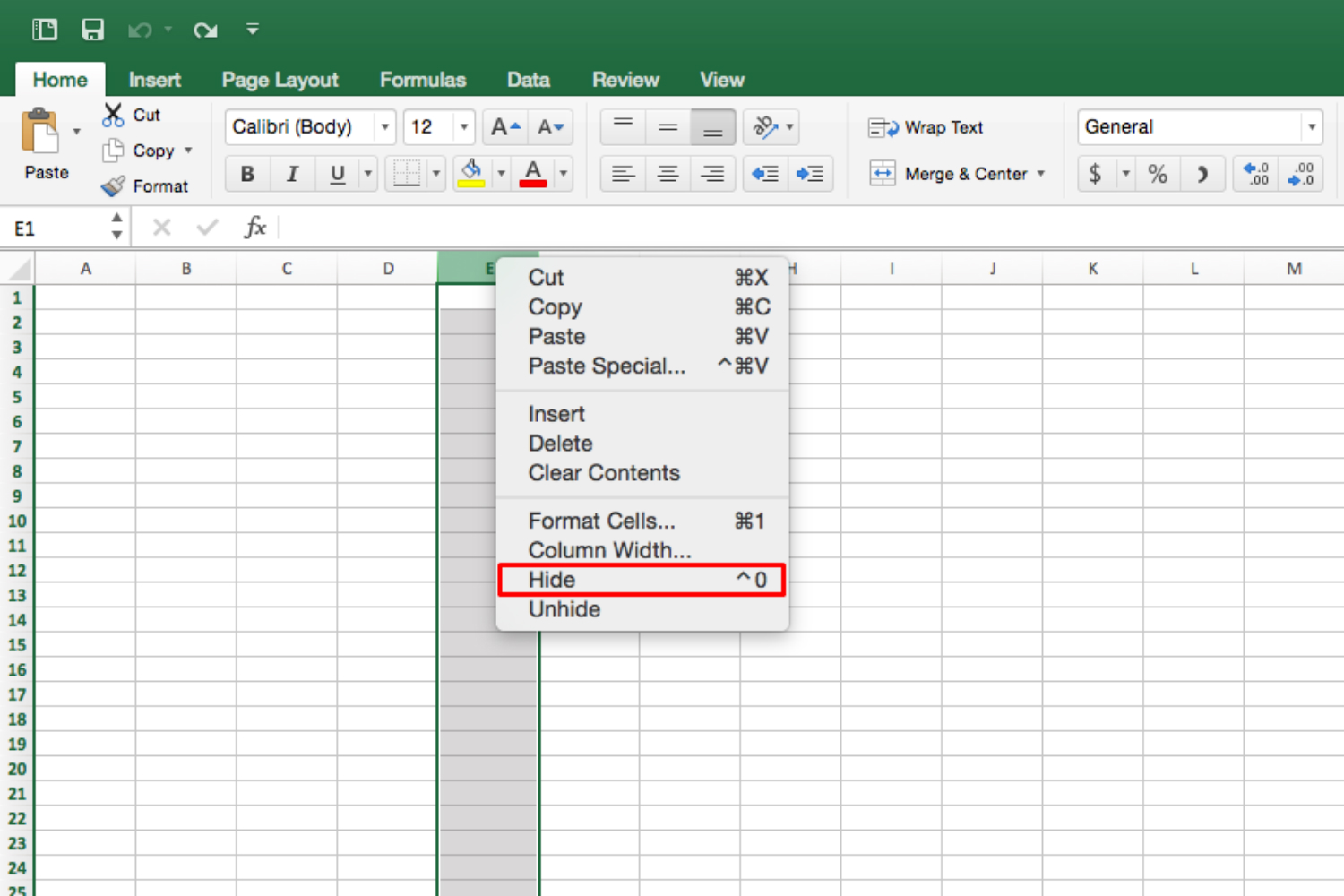
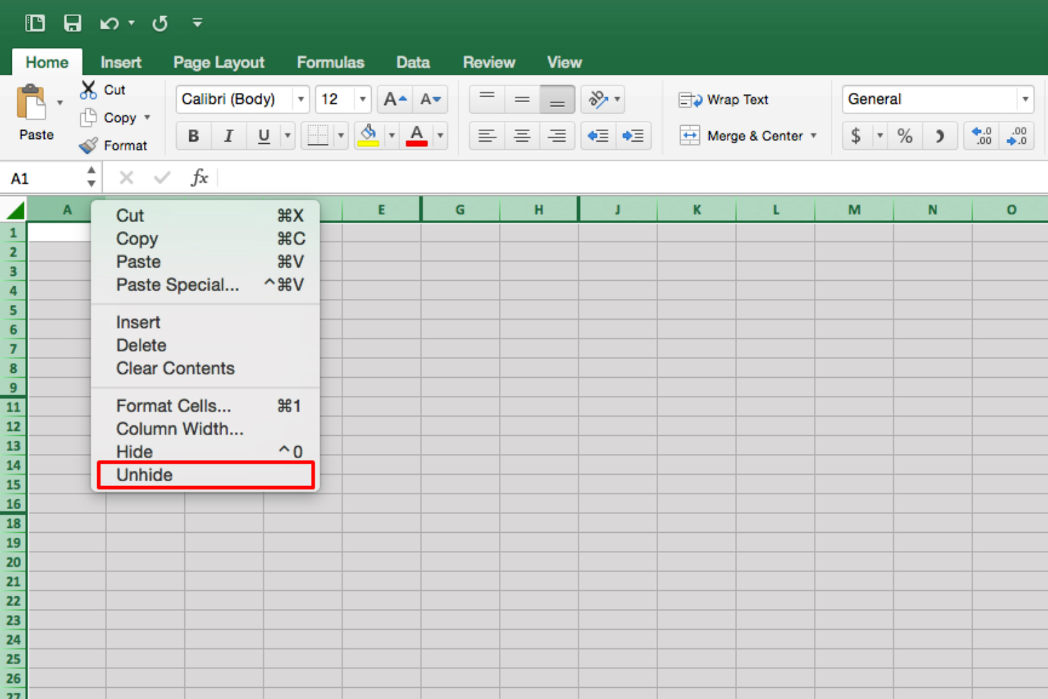
Sometimes, you may want to hide some rows or columns of data. This can be handy if you want to print copies for a presentation, for instance, but the audience only needs to see the essentials. Thankfully, it’s easy to hide a row or column in Excel. Just right-click it, then select Hide.
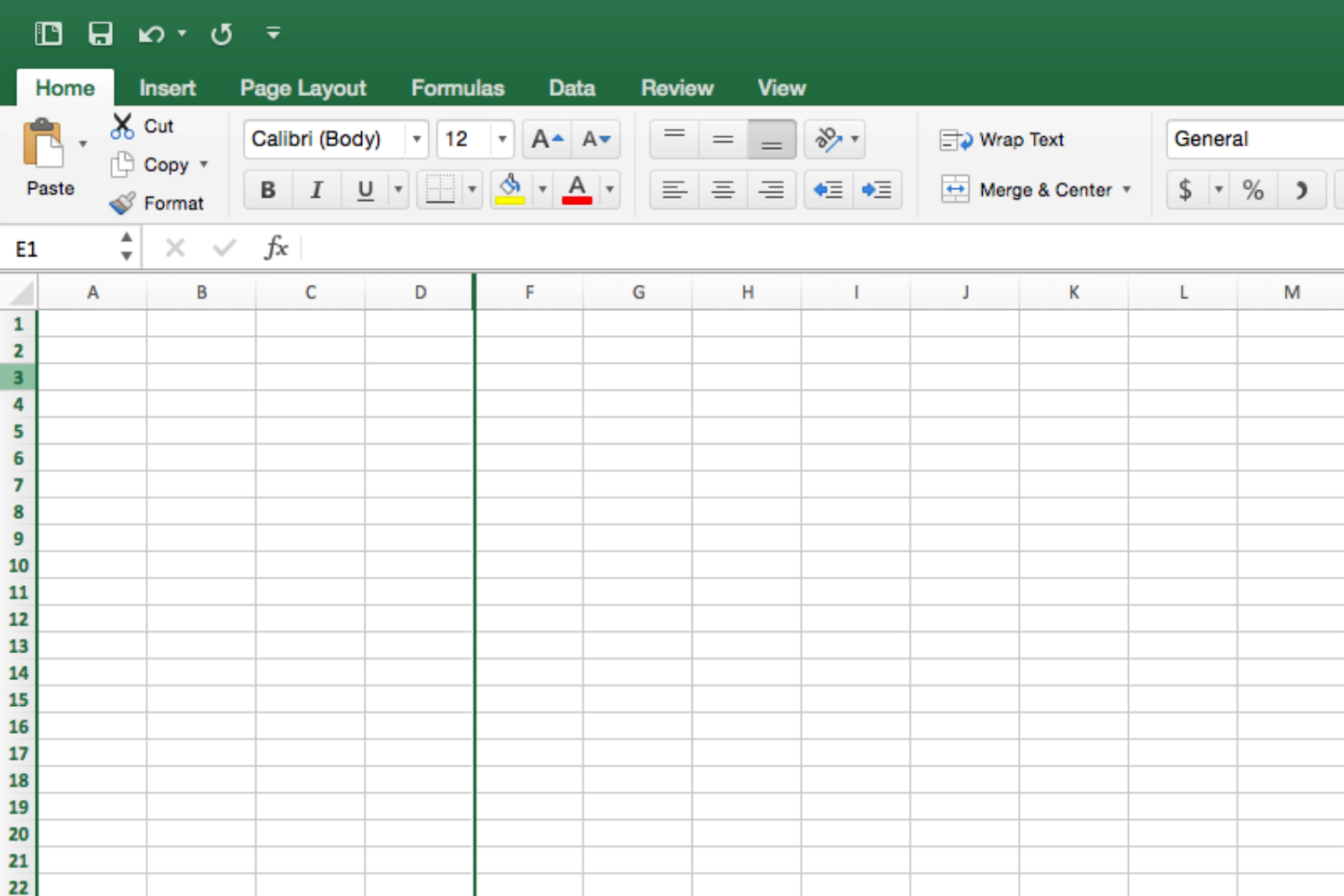
The column or row will be noted by a thick border between the adjacent columns or rows.
If you want to unhide a specific row or column, you will need to highlight the columns or rows on either side of it. Once done, right-click and select Unhide from the resulting list of options.
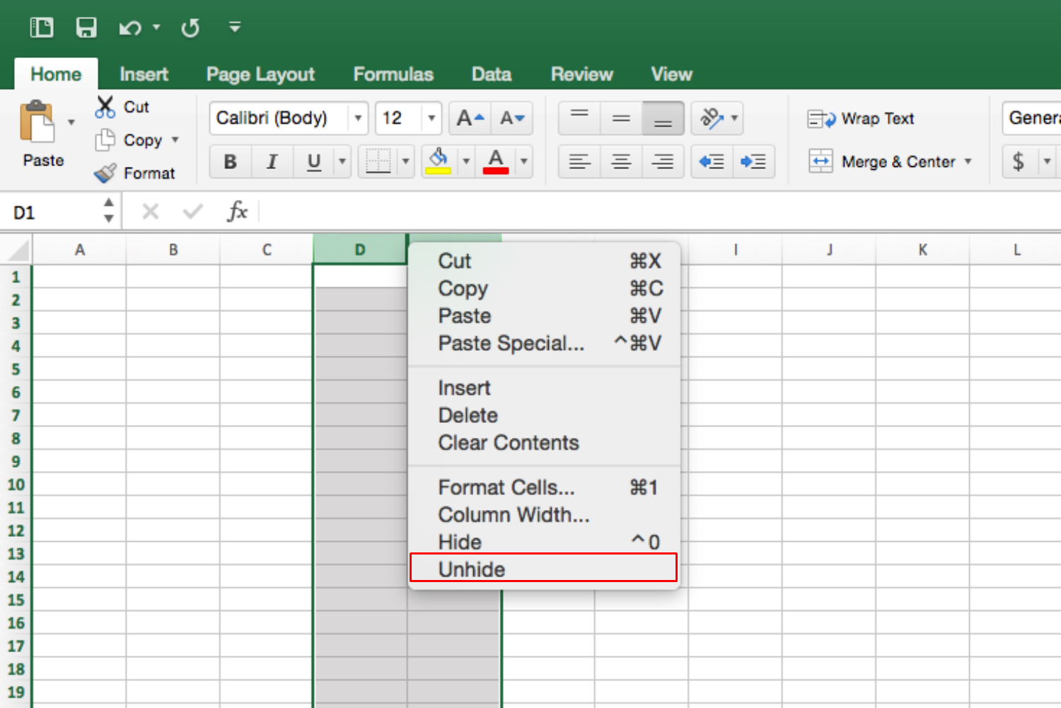
If you have hidden multiple rows and/or columns, you can quickly unhide them by selecting the rows or columns in question, then right-clicking and selecting Unhide. Note: If you’re trying to unhide both rows and columns, you will need to unhide one axis at a time.
How to use vlookup
Sometimes, you may want to ability to retrieve information from a particular cell. Say, for example, you have an inventory for a store, and want to check the price of a particular item. Luckily, you can do so using Excel’s vlookup function.
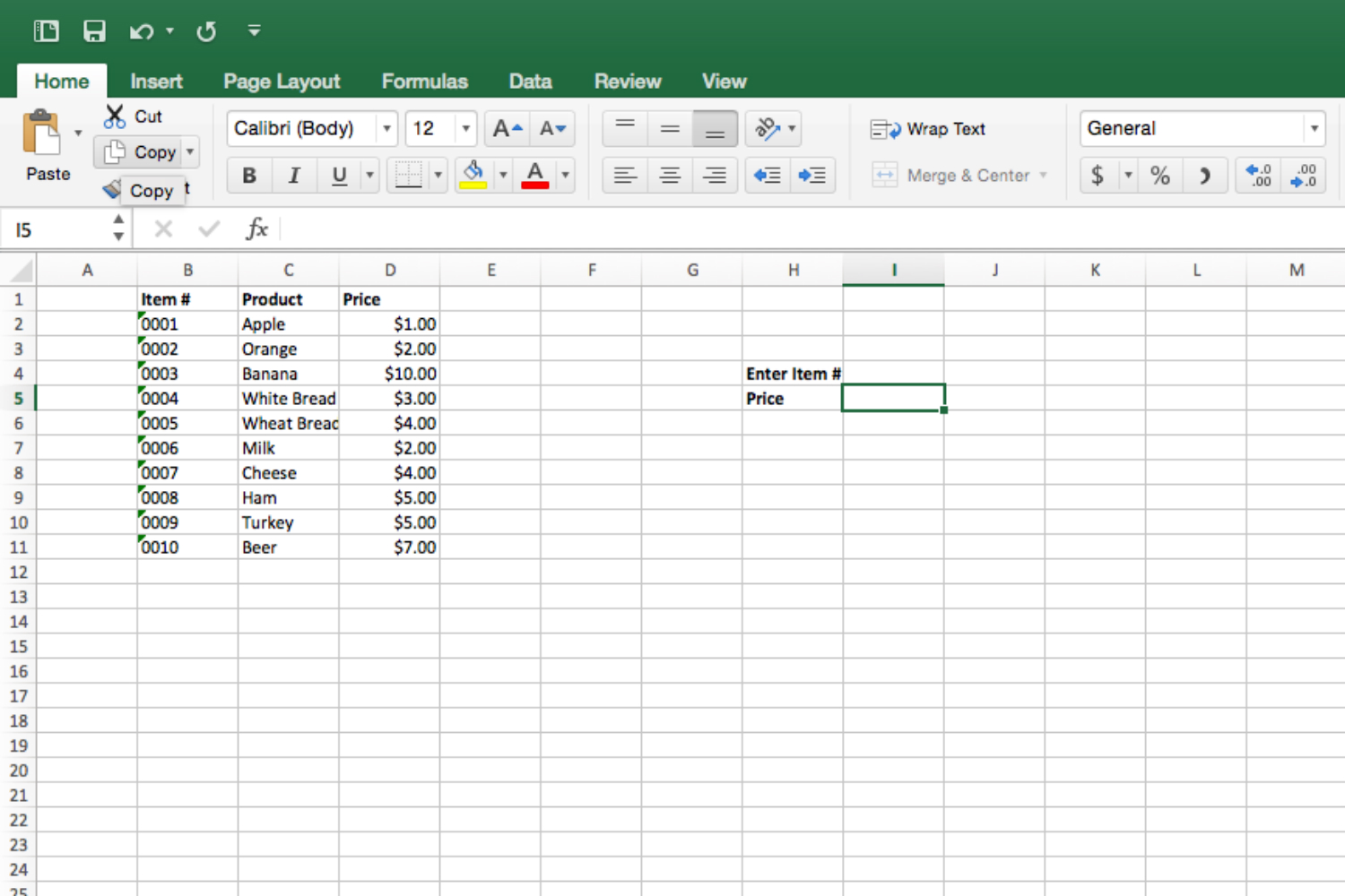
In this example, we have an inventory where every item has an ID number and a price. We want to create a function where users can punch in the ID and get the price automatically. The vlookup function does this, letting you specify a range of columns containing relevant data, a specific column to pull the output from, and a cell to deliver the output to.
We’re going to write the vlookup function in cell I4; this is where the data will be shown. We use cell I3 as the place to input the data, and tell the function that the relevant table runs from B2 to D11, and that the answers will be in the third column (vlookup reads from left to right).

So, our function will be formatted like so: “=vlookup (input cell, range of relevant cells, column to pull answers from),” or “=vlookup(I3,B2:D11,3).”
How to create a drop-down list
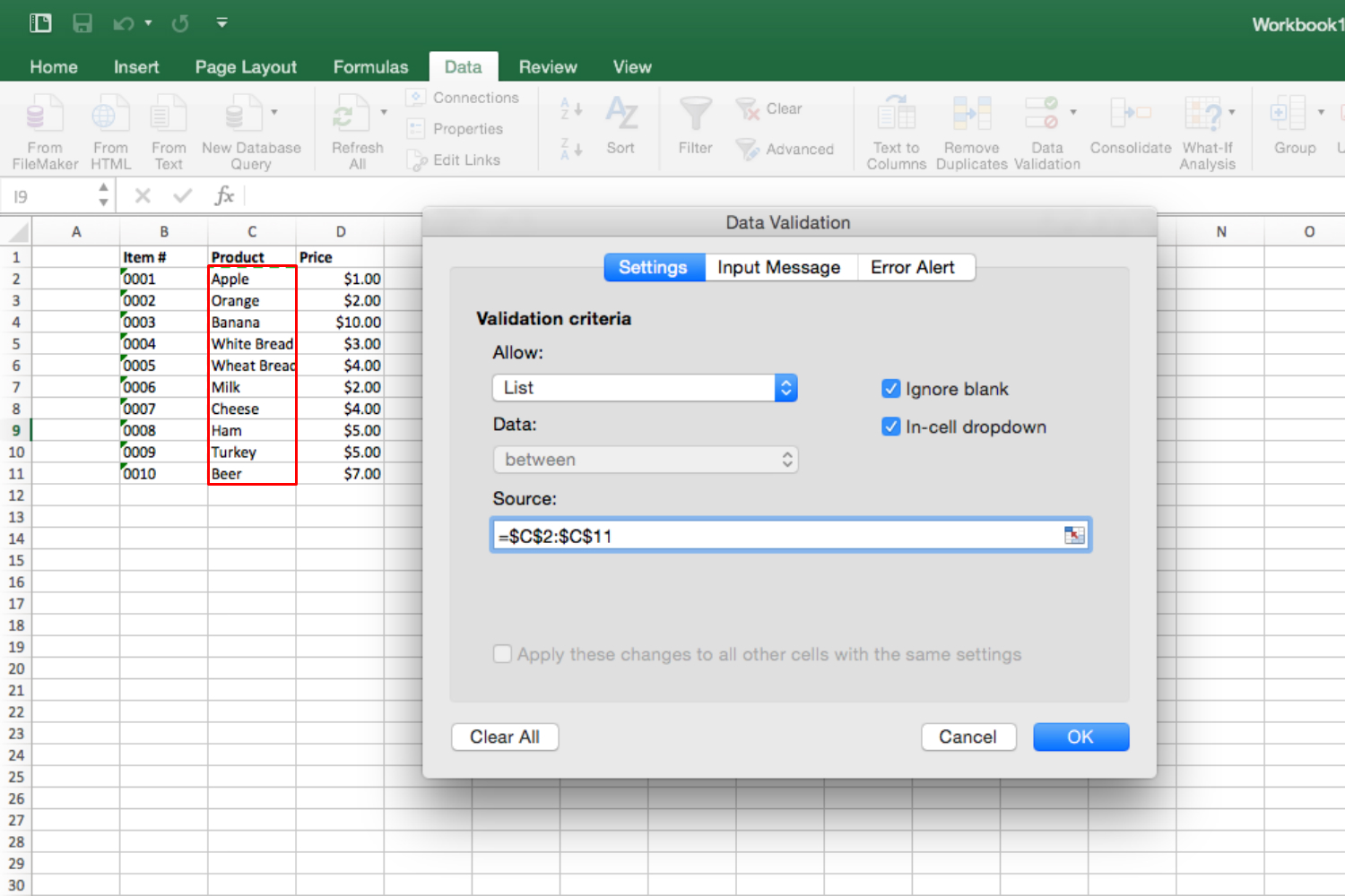
If you want to restrict the range of options a user can put into a cell, a drop-down menu is a good solution. Thankfully, you can easily create one that offers users a list of options to choose from. To start, choose a cell, then go to the Data tab and select Validate.
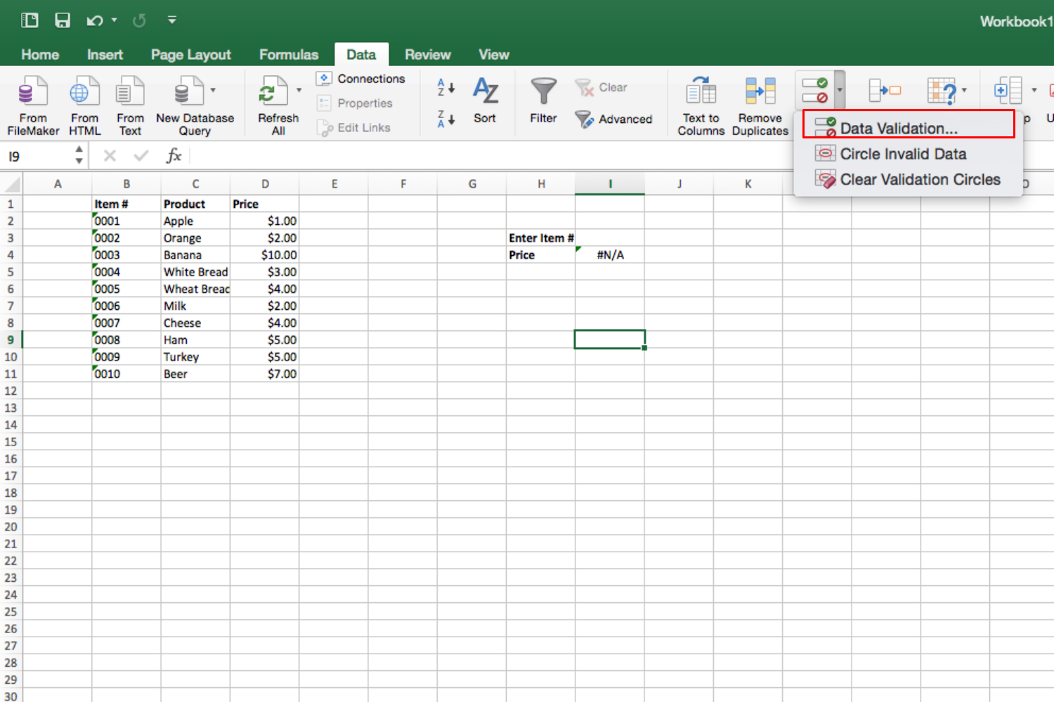
Under Settings, find the drop-down menu labeled Allow. Then, select List.
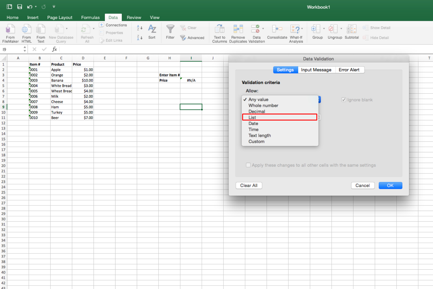
Now, highlight the the cells you want users to choose from and click OK.
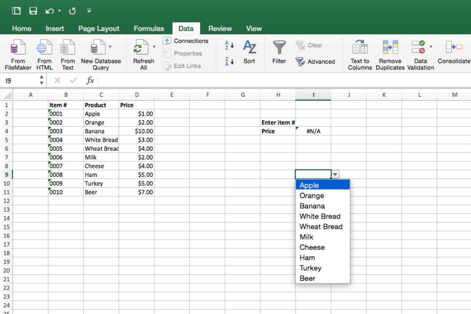
Now, when users click on the cell, they can choose options from a drop-down menu.
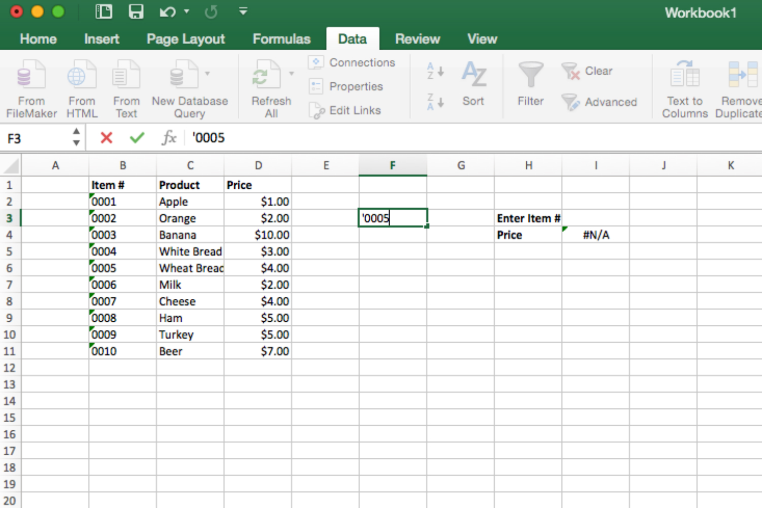
Keep your zeroes visible
Sometimes, you may want to enter strings of numbers beginning with one or more zeroes. Unfortunately, Excel may not show these zeroes, by default. To fix this, add a single quotation mark before the zeroes, e.g. “‘00001” instead of “00001.”
How to concatenate
Sometimes, you may want to reorganize data and combine info from different cells into one entry. You can do this using the concatenate function.
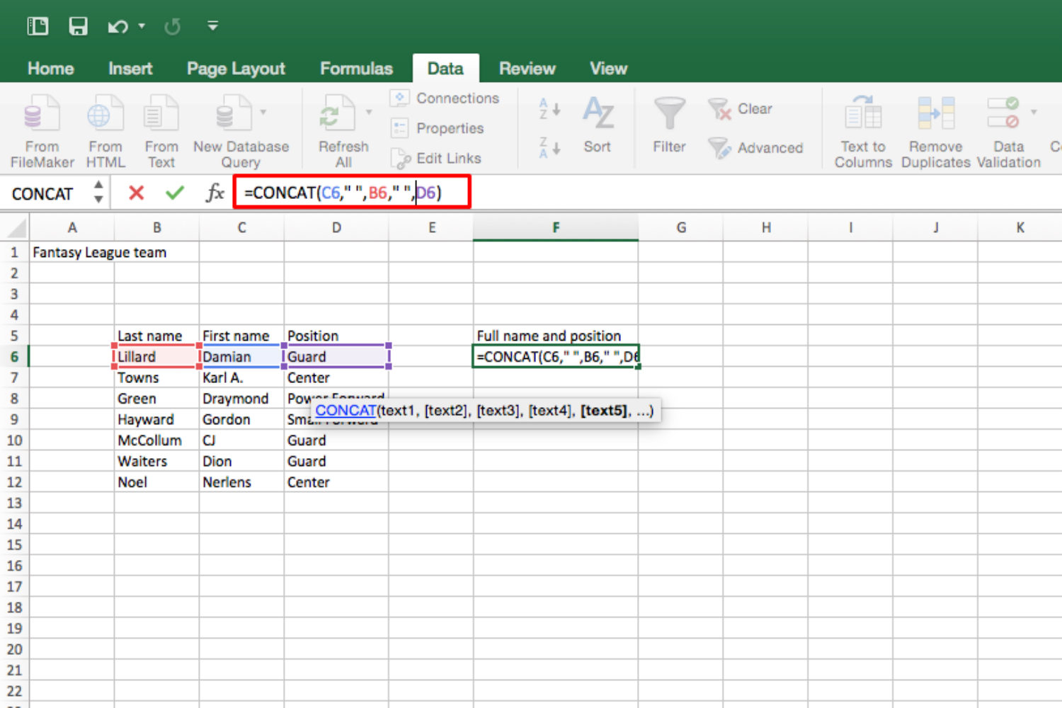
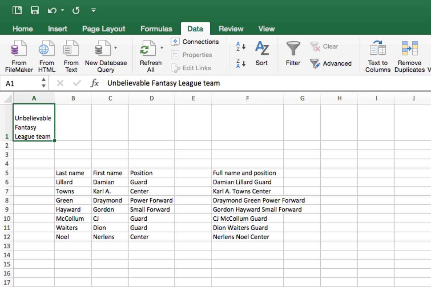
In this example, we have a basketball fantasy league roster, with fields for players’ last names, first names, and positions. If we want to combine all that information in one field, we will need a formula that reads “=concat(first cell, second cell, third cell),” or, in this case, “=concat(C6,B6,D6)” without the quotes.
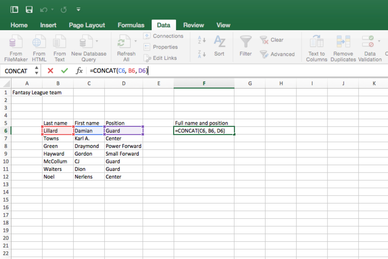
Unfortunately, concatenate doesn’t automatically put spaces between text from different cells. To make a space appear, you will need to add quotation marks with a space in between. Now the function should read “=concat(C6,” “,B6,” “,D6).”
To apply this formula to all the rows we need, click the blue box in the corner of the cell and drag down.
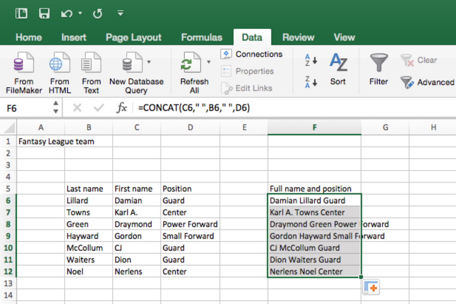
Excel will automatically copy the formula and fill in appropriately.
How to wrap text
Got a lot of text in a single cell? It will probably spill into other cells, which might not look as nice as you’d like. Thankfully, it is easy to make text wrap within a cell.
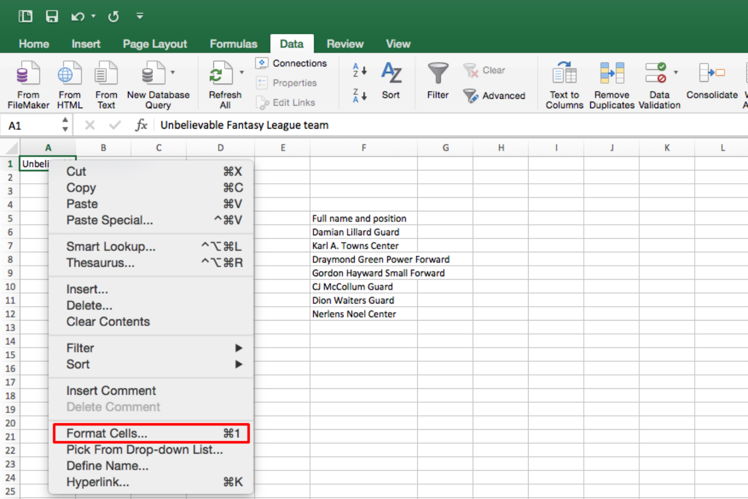
Start by selecting the cell with the excessive text in it. Right-click and select Format cells.
Under the Alignment tab, check the box beside Wrap text.
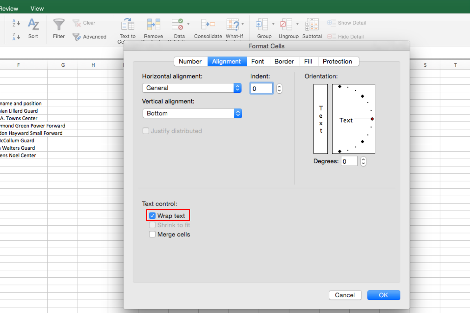
Adjust the width of the cell to your liking.
How to see the developer tab
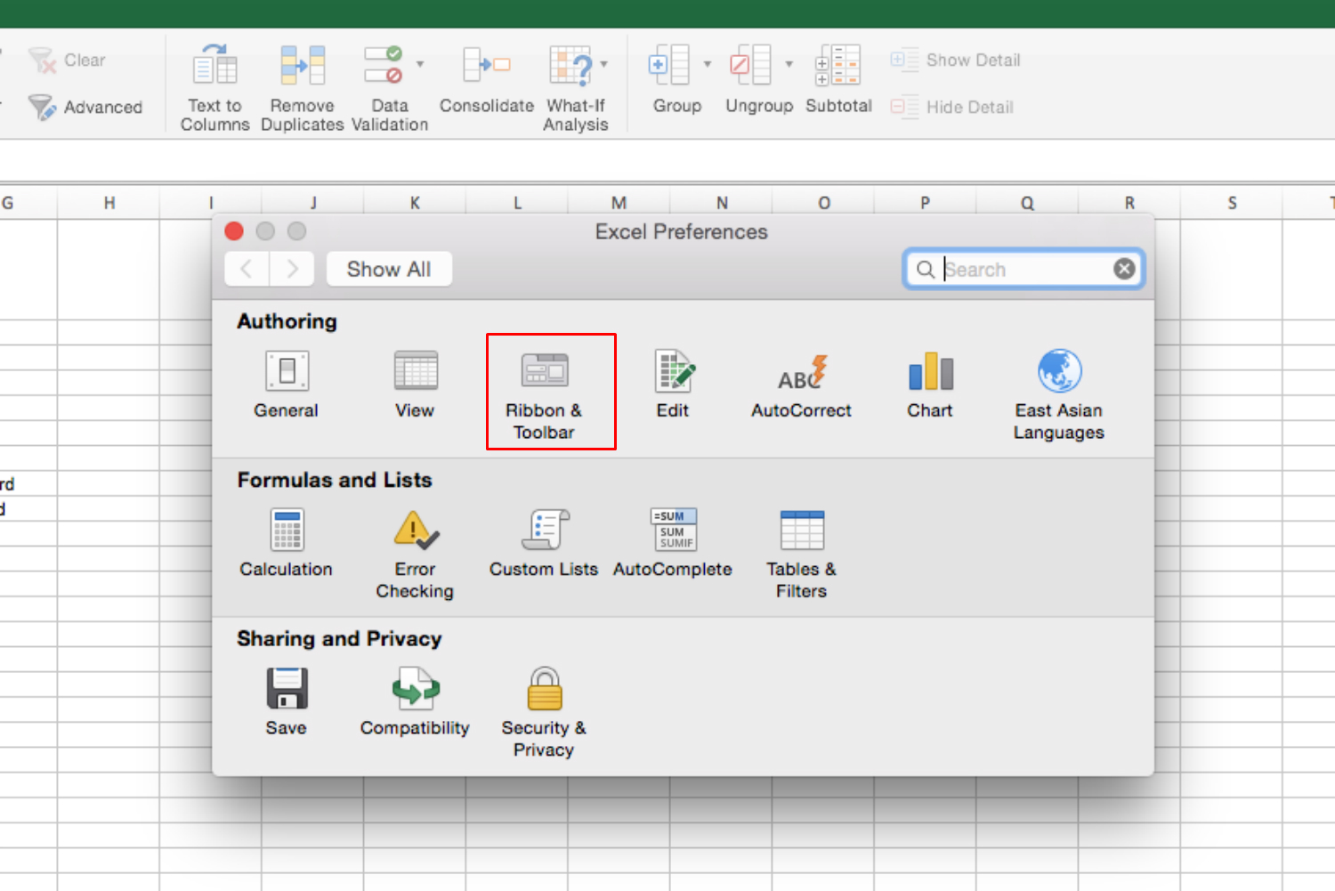
If you want to do more advanced work in Excel — such as create macros — you will need to access the Developer ribbon. Sadly, this tab is hidden by default. To view it, click Excel in the upper-left corner and select Preferences.

Next, click the Ribbon button.
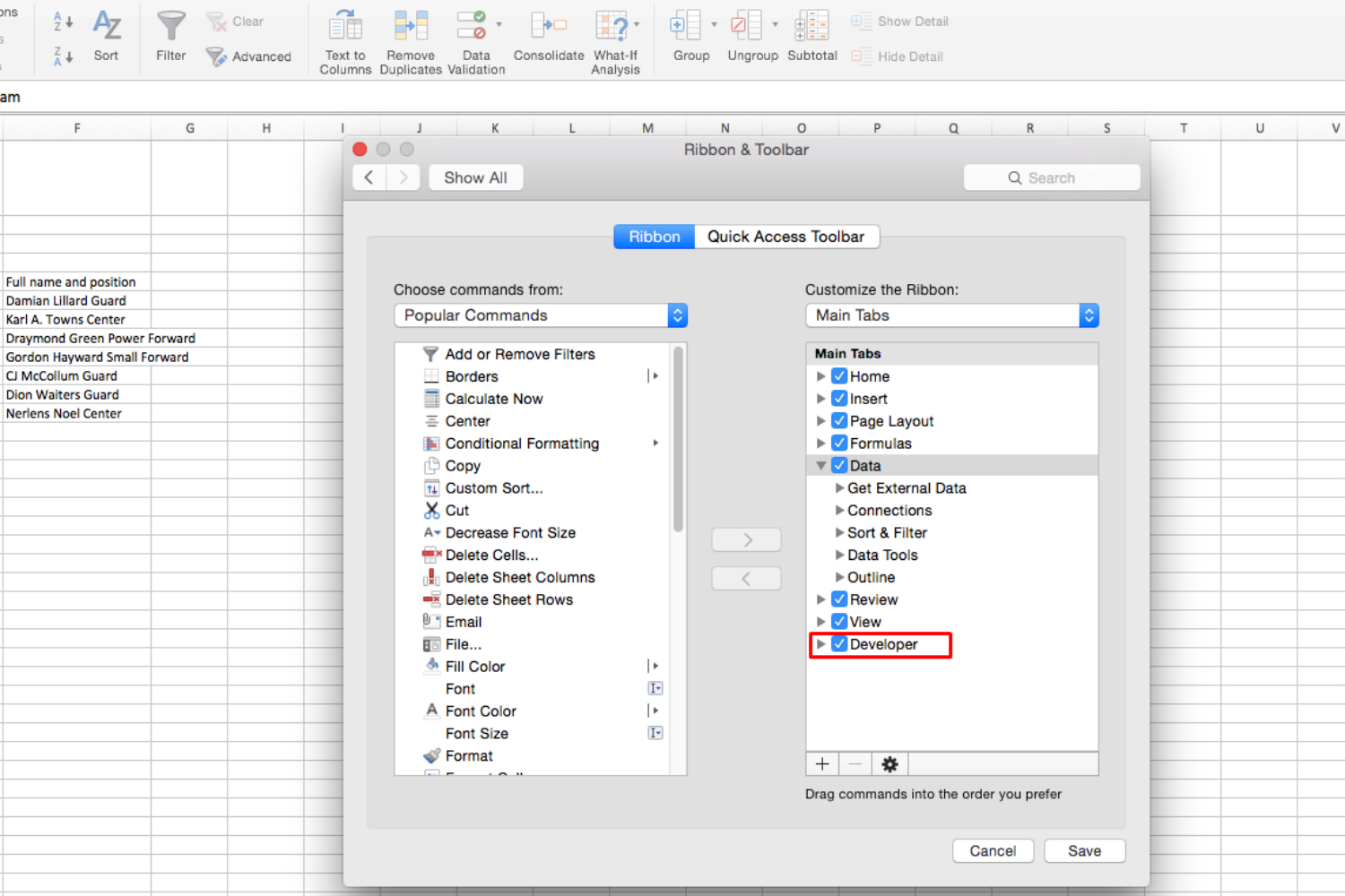
You should see list of buttons, and checkboxes that determine whether you can see the various components. Here, scroll down to the Developer box and check it.
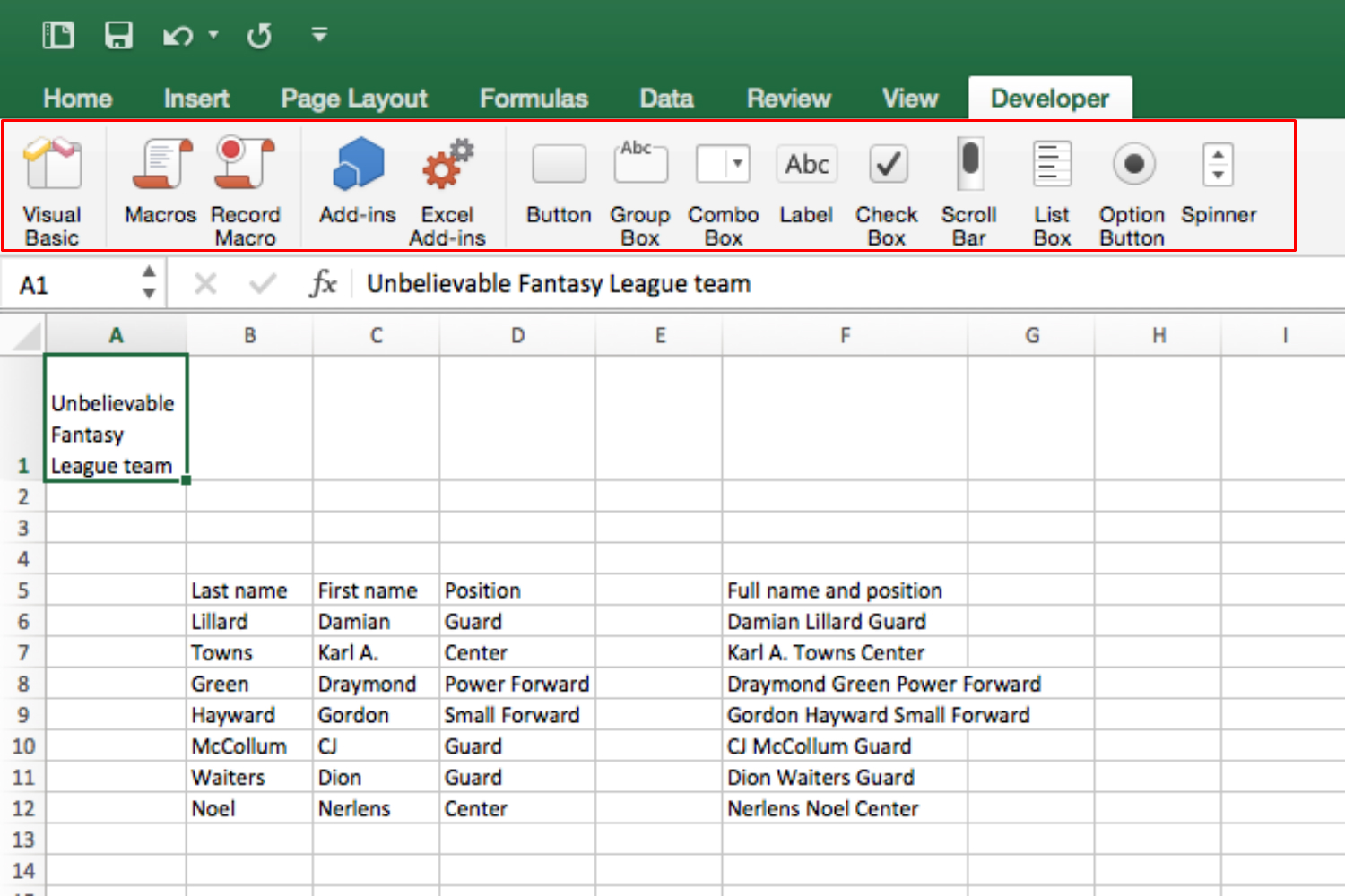
Now you should see the Devolper ribbon at the top.
Editors' Recommendations
- Windows 11 tips and tricks: 8 hidden settings you need to try
- Microsoft Copilot: tips and tricks for using AI in Windows
- Linus Tech Tips restored after crypto scam hack
- How to use iCloud for backups on your iPhone, iPad, or Mac
- Google Meet tips and tricks