So, you want to know how to create a scatter plot in Excel. Chances are, you probably already know what the term means, but given Microsoft Excel’s arsenal of options packed into each tab, getting started can be somewhat daunting, especially for Excel newcomers. The process isn’t quite as hard as it sounds, but you’ll need to understand exactly what you want before you go digging through Excel’s extended toolset.
That said, scatter plots are limited in how data is presented. If you’re looking for a chart using lots of text, a line chart might be a more appropriate option for your needs. You can use text labels along the horizontal axis in a line chart, as well as a time scale. Regardless, here is our guide to get you started on creating a scatter plot in the latest version of Excel and you can decide later if a different chart style is in order.
Grab your data
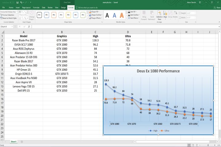
In our demo, we wanted to see how 12 laptops performed when we benchmarked their hardware with an extremely taxing PC game. Our data includes the types of discrete graphics chips installed in each model and the average framerate generated by each using high and ultra detail settings when benchmarking the game at 1080p. The chart will be simple so you can get the hang of creating a scatter plot quickly.
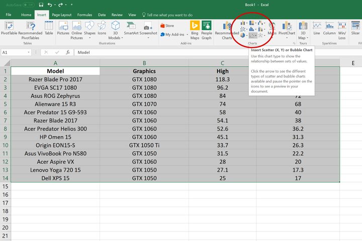
First, select all the data you want to include in the chart. After that, click on the Insert tab and navigate to the Charts section in the middle of Excel’s ribbon. The Scatter button is hard to see in the most recent version of Excel, which resides between the Pie/Donut button, and the web-like Surface/Radar button (see above). A drop-down menu will then appear to present five scatter-based styles:
- Scatter (dots only)
- Scatter with smooth lines and markers
- Scatter with smooth lines (no markers)
- Scatter with straight lines and markers
- Scatter with straight lines (no markers)
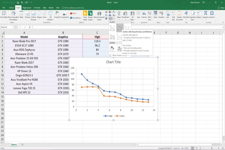
Because the scatter chart only plots numbers, the points and lines will be based on the columns of numbers you chose to plot. For instance, our chart renders two lines with 13 points each: The blue line charts our “high” data, and an orange line charts our “ultra” data. The chart may appear over your Excel sheet’s raw data once it’s generated, but you can easily move it anywhere on the sheet by clicking on the chart, and then holding down the mouse button while you drag the cursor across the screen.
Be creative with the scatter chart
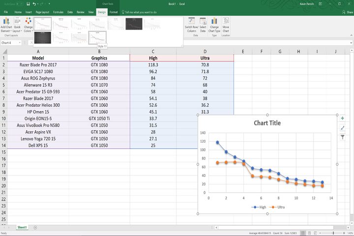
With the chart created, Excel defaults to the Design tab on the ribbon. Here, you have a choice of 11 visual styles via the Quick Layout option. You also see the Change Colors button as well, enabling you to select one of four “colorful” color schemes/pallets or one of 13 “monochromatic” pallets. As shown above, we chose Style 11 because it gives the lines and dots visual depth but we kept the color scheme unchanged. All the basics of creating a graph in Excel apply.
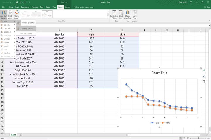
For our chart, we didn’t want the horizontal lines nor the numbers stacked on the left. To remove the numbers, we made the ribbon’s Design tab active, and then clicked the Add Chart Element button listed above Chart Layouts. After that, we chose Axis, and then deselected Primary Vertical. As shown above, this method removed all the numbers on the left but kept the numbers running along the bottom intact. Note that the Primary Horizontal icon remains gray, indicating its active state.
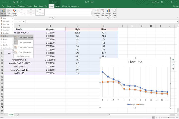
To remove the horizontal lines, we clicked Add Chart Element again, but this time scrolled down to the Gridlines option. Here, all you need to select is Primary Major Horizontal to turn off the horizontal lines, but make sure Primary Major Vertical is highlighted in gray so that the vertical lines remain.
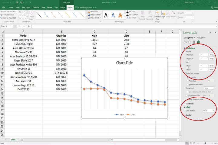
But the vertical lines still aren’t right — we want a line to represent each laptop even though we can’t inject text into its root. To solve this, we clicked Add Chart Element again, then Axis, and then More Axis Options. The Format Axis panel appeared on the right providing four sections, and the first section — Axis Options — expanded by default. Here we set the Major and Minor units to 1.0 so we’re counting each laptop, and the Bounds minimum to 1.0 and the Bounds maximum to 13.0 so we actually have 13 lines from left to right.
Because we can’t assign laptop names or graphic chip labels to the base of each line, we removed the numbers at the bottom, aka the horizontal value axis, or X-axis. To do this, we stayed on the Format Axis panel, and expanded the Labels category towards the bottom. Here we merely chose None as the Label Position as shown in the second circle in the screenshot above, which removed the unnecessary horizontal numbers.

Other pretty things
Of course, to change the chart’s heading, simply double-click on it to edit the text. This will produce the Format Chart Title panel on the right so you can spruce the heading up with a background fill or border. You can do something similar with the chart itself by double-clicking anywhere on the chart to pull up the Format Chart Area panel on the right. In our case, we went with a solid blue line with a width of two points so it stands out on the sheet. We also gave it a cool blue gradient fill to spruce it up with some color, but you can use fills based on solids, patterns, textures, and pictures as well.
But using a gradient meant we lost the lines in the blue background. To change the color of your grid lines, simply click on them within your chart to produce the Format Major Gridlines panel on the right. Here you can set the type of lines you want to use, their transparency, width, color, and so on. Since we didn’t need to see the sole horizontal line along the bottom, we clicked on it to produce the Format Axis panel again and chose No line to remove it.
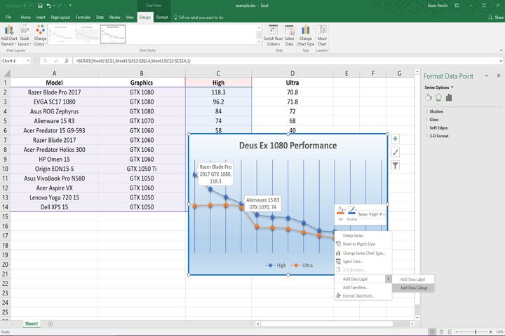
But we still can’t tell what’s what on the chart — it’s all just dots and lines. Thankfully, you can show data in several ways. In one example, we could click on one of the points to activate it, and then right-click on it to access the Add Data Label option. You can choose to show the number data associated with that point (the average frames per second in our case), or show all the data associated with that point along the X-axis. For our chart, we did this with three points to show the performance difference when switching internal graphics.
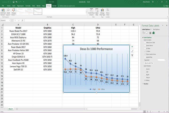
Another example would be to simply show the number data of each point. Click on a point on the chart again to activate it, right-click to show the Add Data Labels option again, and then select Add Data Labels in the rollout menu. The numbers will appear and can be visually altered using the Format Data Labels panel on the right. Here you can re-position the labels, add or remove the data from other cells, and change the thickness of the text.
Be a cheater… it’s OK
So while we now have the average frame rates for each plot on the chart, we still can’t see the hardware that was used. Even more, we can’t use text as data along the bottom of the chart, but we can put the horizontal axis title back on our chart and “cheat.” Unfortunately, the axis title text box doesn’t completely extend from one side of the chart to the other (it’s locked by an algorithm, says Microsoft), so we entered text and used spaces to get a general idea of the major changes in hardware. It’s not exactly what we wanted, but it will do given the scatter chart’s limitations.
Finally, many visual elements can be altered on your chart using tools supplied on the Format tab when your chart is highlighted. What you alter depends on what is selected in the Current Selection area on Excel’s ribbon, such as Horizontal (Value) Axis Title when manipulating the horizontal text as we just did. You’ll see options for selecting a bounding box, text styles, text effects, and more. Alternatively, you can right-click on anything within the chart to pull up the option for modifying that element. In the case of horizontal axis title, you can quickly fill the text box, create an outline, or select from a large collection of styles.
This is just one of many Excel charts
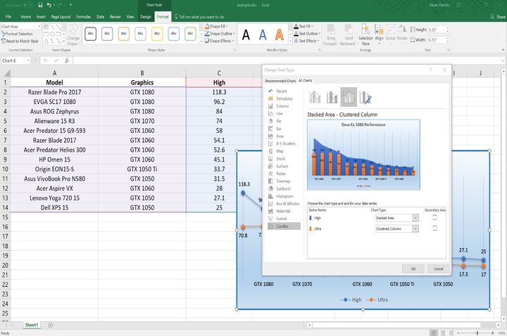
A scatter plot is just one style of chart-making in Excel. If you find that you need more flexibility in the presentation, you can right-click on the chart and select Change chart type. Here, you will see a list of all the charts Excel supports and previews of how your data will be used for each type. These styles include Column, Line, Bar, and even templates you used or downloaded in the past. There’s a “Combo” option too for using multiple styles on one chart.
Have fun with your scatter plot. This was just one example of how to use this feature, and could be put to better use, such as tracking the amount of rainfall for seven days, the growth of various plants over a month’s time, forecasting the company’s growth based on current sales numbers, and so on. But again, a scatter plot deals with numeric data such as dates, times, currencies, percentages, and so on. It’s capable of showing text related to those numbers but the horizontal and vertical values can’t use text. If that’s what you’re looking for, a line chart would be more appropriate.
For more tips and tricks to make your Excel experience better, check these Microsoft Excel tips and tricks.